cosine bell

description

The cosine_bell/convergence_* and cosine_bell/convergence_*/with_viz tasks implement the Cosine Bell test case as first described in Williamson et al. 1992 but using the variant from Sec. 3a of Skamarock and Gassmann. A flow field representing solid-body rotation transports a bell-shaped perturbation in a tracer \(\psi\) once around the sphere, returning to its initial location.

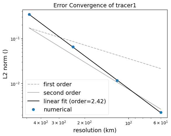
The convergence_both task is a convergence test with time step varying proportionately to cell size, while convergence_time and convergence_space vary only the time step and the cell size, respectively. The result of the analysis step of each task is a plot like the following showing convergence as a function of the cell size and/or the time step:

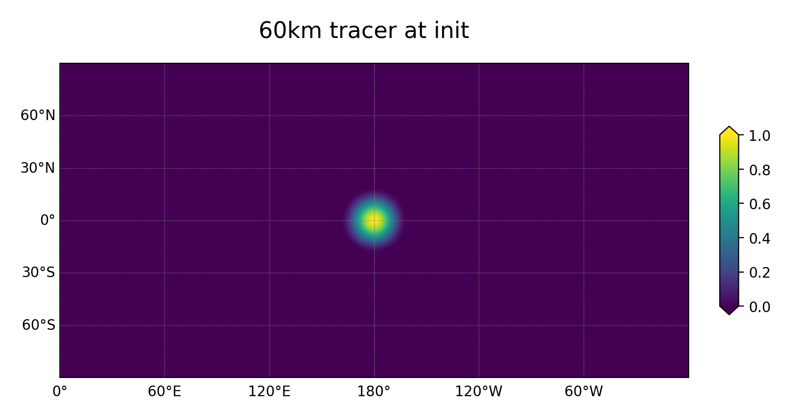
The with_viz variant also includes visualization of the initial and final state on a lat-lon grid for each resolution. The visualization is not included in the other versions of the task in order to not slow down regression testing.

Another task, cosine_bell/decomp, performs two runs of the Cosine Bell test at coarse resolution, once with 12 and once with 24 cores, to verify the bit-for-bit identical results for tracer advection across different core counts.

A final task, cosine_bell/restart, performs two time steps of the Cosine Bell test at coarse resolution, then performs reruns the second time step, as a restart run to verify the bit-for-bit restart capability for tracer advection.

suppported models

These tasks support both MPAS-Ocean and Omega.

mesh

Two global mesh variants are tested, quasi-uniform (QU) and icosohydral. There are also variants to test convergence in space, time, or both space and time as well as the restart test. In addition, the tests can be set up with or without the viz step. Thus, there are 14 variants of the task:

ocean/spherical/icos/cosine_bell/convergence_space
ocean/spherical/icos/cosine_bell/convergence_space/with_viz
ocean/spherical/icos/cosine_bell/convergence_time
ocean/spherical/icos/cosine_bell/convergence_time/with_viz
ocean/spherical/icos/cosine_bell/convergence_both
ocean/spherical/icos/cosine_bell/convergence_both/with_viz
ocean/spherical/icos/cosine_bell/decomp
ocean/spherical/icos/cosine_bell/restart
ocean/spherical/qu/cosine_bell/convergence_space
ocean/spherical/qu/cosine_bell/convergence_space/with_viz
ocean/spherical/qu/cosine_bell/convergence_time
ocean/spherical/qu/cosine_bell/convergence_time/with_viz
ocean/spherical/qu/cosine_bell/convergence_both
ocean/spherical/qu/cosine_bell/convergence_both/with_viz
ocean/spherical/icos/cosine_bell/decomp
ocean/spherical/qu/cosine_bell/restart

The default resolutions used in the task depends on the mesh type.

For the icos mesh type, the defaults are 60, 120, 240, 480 km, as determined by the following config options. See Convergence Tests for more details.

# config options for spherical convergence tests
[spherical_convergence]

# The base resolution for the icosahedral mesh to which the refinement
# factors are applied
icos_base_resolution = 60.

# a list of icosahedral mesh resolutions (km) to test
icos_refinement_factors = 8., 4., 2., 1.
# a list of icosahedral mesh resolutions (km) to test

For the qu mesh type, they are 60, 90, 120, 150, 180, 210, 240 km as determined by the following config options:

# config options for spherical convergence tests
[spherical_convergence]

# The base resolution for the quasi-uniform mesh to which the refinement
# factors are applied
qu_base_resolution = 120.

# a list of quasi-uniform mesh resolutions (km) to test
qu_refinement_factors = 0.5, 0.75, 1., 1.25, 1.5, 1.75, 2.

To alter the resolutions used in the convergence tasks, you will need to create your own config file (or add a spherical_convergence section to a config file if you’re already using one). The resolutions are a comma-separated list of the resolution of the mesh in km. If you specify a different list before setting up cosine_bell, steps will be generated with the requested resolutions. (If you alter icos_resolutions or qu_resolutions in the task’s config file in the work directory, nothing will happen.) For icos meshes, make sure you use a resolution close to those listed in Spherical Meshes. Each resolution will be rounded to the nearest allowed icosahedral resolution.

The base_mesh steps are shared with other tasks so they are not housed in the cosine_bell work directory. Instead, they are in work directories like:

ocean/spherical/icos/base_mesh/60km
ocean/spherical/qu/base_mesh/60km

For convenience, there are symlinks inside of the cosine_bell and cosine_bell/with_viz work directories, e.g.:

ocean/spherical/icos/cosine_bell/base_mesh/60km
ocean/spherical/qu/cosine_bell/base_mesh/60km
ocean/spherical/icos/cosine_bell/with_viz/base_mesh/60km
ocean/spherical/qu/cosine_bell/with_viz/base_mesh/60km

vertical grid

This task only exercises the shallow water dynamics. As such, a single vertical level may be used. The bottom depth is constant and the results should be insensitive to the choice of bottom_depth.

# Options related to the vertical grid
[vertical_grid]

# the type of vertical grid
grid_type = uniform

# Number of vertical levels
vert_levels = 1

# Depth of the bottom of the ocean
bottom_depth = 300.0

# The type of vertical coordinate (e.g. z-level, z-star)
coord_type = z-level

# Whether to use "partial" or "full", or "None" to not alter the topography
partial_cell_type = None

# The minimum fraction of a layer for partial cells
min_pc_fraction = 0.1

initial conditions

The initial bell is defined by any passive tracer \(\psi\):

\[\begin{split} \psi = \begin{cases} \left( \psi_0/2 \right) \left[ 1 + \cos(\pi r/R )\right] & \text{if } r < R \\ 0 & \text{if } r \ge R \end{cases} \end{split}\]

where \(\psi_0 = 1\), the bell radius \(R = a/3\), and \(a\) is the radius of the sphere. psi_0 and radius, \(R\), are given as config options and may be altered by the user. In the init step we assign debug_tracers_1 to \(\psi\).

The initial velocity is equatorial:

\[ u_0 = 2 \pi a/ \tau \]

Where \(\tau\) is the time it takes to transit the equator. The default is 24 days, and can be altered by the user using the config option vel_pd.

Temperature and salinity are not evolved in this task and are given constant values determined by config options temperature and salinity.

The Coriolis parameters fCell, fEdge, and fVertex do not need to be specified for a global mesh and are initialized as zeros.

forcing

N/A. This case is run with all velocity tendencies disabled so the velocity field remains at the initial velocity \(u_0\).

time step and run duration

This task uses the Runge-Kutta 4th-order (RK4) time integrator. The time step for forward integration is determined by multiplying the resolution by a config option, rk4_dt_per_km, so that coarser meshes have longer time steps. You can alter this before setup (in a user config file) or before running the task (in the config file in the work directory).

# config options for convergence tests
[convergence_forward]

# time integrator: {'split_explicit', 'RK4'}
time_integrator = RK4

# RK4 time step per resolution (s/km), since dt is proportional to resolution
rk4_dt_per_km = 3.0

The convergence_eval_time, run_duration and output_interval are the period for advection to make a full rotation around the globe, 24 days:

# config options for convergence forward steps
[convergence_forward]

# Run duration in hours
run_duration = ${cosine_bell:vel_pd}

# Output interval in hours
output_interval = ${cosine_bell:vel_pd}

Here, ${cosine_bell:vel_pd} means that the same value is used as in the option vel_pd in section [cosine_bell], see below.

config options

The cosine_bell config options include:

# options for cosine bell convergence test case
[cosine_bell]

# the constant temperature of the domain
temperature = 15.0

# the constant salinity of the domain
salinity = 35.0

# the central latitude (rad) of the cosine bell
lat_center = 0.0

# the central longitude (rad) of the cosine bell
lon_center = 3.14159265

# the radius (m) of cosine bell
radius = 2123666.6667

# hill max of tracer
psi0 = 1.0

# time (hours) for bell to transit equator once
vel_pd = 576.0

# convergence threshold below which the test fails
convergence_thresh = 1.8


# options for visualization for the cosine bell convergence test case
[cosine_bell_viz]

# visualization latitude and longitude resolution
dlon = 0.5
dlat = 0.5

# remapping method ('bilinear', 'neareststod', 'conserve')
remap_method = conserve

# colormap options
# colormap
colormap_name = viridis

# the type of norm used in the colormap
norm_type = linear

# A dictionary with keywords for the norm
norm_args = {'vmin': 0., 'vmax': 1.}

# We could provide colorbar tick marks but we'll leave the defaults
# colorbar_ticks = np.linspace(0., 1., 9)

The 7 options from temperature to vel_pd are used to control properties of the cosine bell and the rest of the sphere, as well as the advection.

The option convergence_thresh is a threshold for determining when the convergence rates are not above a minimum convergence rate.

The options in the cosine_bell_viz section are used in visualizing the initial and final states on a lon-lat grid for cosine_bell/with_viz tasks.

By default, the convergence analysis step analyzes convergence after the cosine bell has circulated the globe once. It also computes the L2 norm. Both of these config options can be changed here:

# config options for spherical convergence tests
[convergence]

# Evaluation time for convergence analysis (in days)
convergence_eval_time = ${cosine_bell:vel_pd}

# Convergence threshold below which a test fails
convergence_thresh = ${cosine_bell:convergence_thresh}

# Type of error to compute
error_type = l2

cores

The target and minimum number of cores are determined by goal_cells_per_core and max_cells_per_core from the ocean section of the config file, respectively. This ensures that the number of cells per core is roughly constant across the different resolutions in the convergence study.