correlated tracers 2-d

description

The correlated_tracers_2d and correlated_tracers_2d/with_viz tasks implement the non-divergent flow field test of (1) numerical order of convergence and (2) mixing as described in Lauritzen et al. 2012.

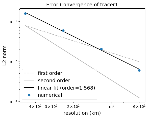
The numerical order of convergence is analyzed in the analysis step and produces a figure similar to the following showing L2 error norm as a function of horizontal resolution:

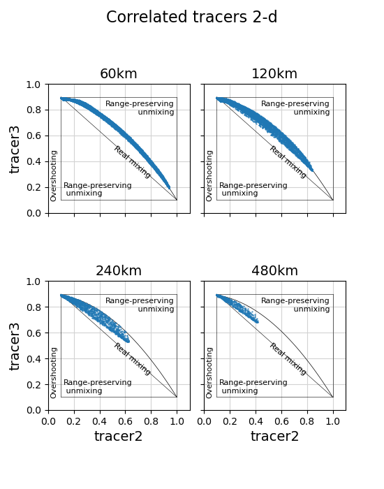
../../../_images/correlated_tracers_2d_convergence.png

The ability of the horizontal advection scheme to maintain nonlinear relationships between tracers is addressed in the mixing_analysis step. This step produces a visualization of the relationship between two debug tracers at the end of the simulation:

../../../_images/correlated_tracers_2d_mixing.png

mesh

Two global mesh variants are tested, quasi-uniform (QU) and icosohydral. Thus, there are 4 variants of the task:

ocean/spherical/icos/correlated_tracers_2d
ocean/spherical/icos/correlated_tracers_2d/with_viz
ocean/spherical/qu/correlated_tracers_2d
ocean/spherical/qu/correlated_tracers_2d/with_viz

The default resolutions used in the task depends on the mesh type.

For the icos mesh type, the defaults are:

# config options for spherical convergence tests
[spherical_convergence]

# a list of icosahedral mesh resolutions (km) to test
icos_resolutions = 60, 120, 240, 480

for the qu mesh type, they are:

# config options for spherical convergence tests
[spherical_convergence]

# a list of quasi-uniform mesh resolutions (km) to test
qu_resolutions = 60, 90, 120, 150, 180, 210, 240

To alter the resolutions used in this task, you will need to create your own config file (or add a spherical_convergence section to a config file if you’re already using one). The resolutions are a comma-separated list of the resolution of the mesh in km. If you specify a different list before setting up correlated_tracers_2d, steps will be generated with the requested resolutions. (If you alter icos_resolutions or qu_resolutions) in the task’s config file in the work directory, nothing will happen.) For icos meshes, make sure you use a resolution close to those listed in Spherical Meshes. Each resolution will be rounded to the nearest allowed icosahedral resolution.

The base_mesh steps are shared with other tasks so they are not housed in the correlated_tracers_2d work directory. Instead, they are in work directories like:

ocean/spherical/icos/base_mesh/60km
ocean/spherical/qu/base_mesh/60km

For convenience, there are symlinks inside of the correlated_tracers_2d and correlated_tracers_2d/with_viz work directories, e.g.:

ocean/spherical/icos/correlated_tracers_2d/base_mesh/60km
ocean/spherical/qu/correlated_tracers_2d/base_mesh/60km
ocean/spherical/icos/correlated_tracers_2d/with_viz/base_mesh/60km
ocean/spherical/qu/correlated_tracers_2d/with_viz/base_mesh/60km

vertical grid

This task only exercises the shallow water dynamics. As such, a single vertical level may be used. The bottom depth is constant and the results should be insensitive to the choice of bottom_depth.

# Options related to the vertical grid
[vertical_grid]

# the type of vertical grid
grid_type = uniform

# Number of vertical levels
vert_levels = 3

# Depth of the bottom of the ocean
bottom_depth = 300.0

# The type of vertical coordinate (e.g. z-level, z-star)
coord_type = z-level

# Whether to use "partial" or "full", or "None" to not alter the topography
partial_cell_type = None

# The minimum fraction of a layer for partial cells
min_pc_fraction = 0.1

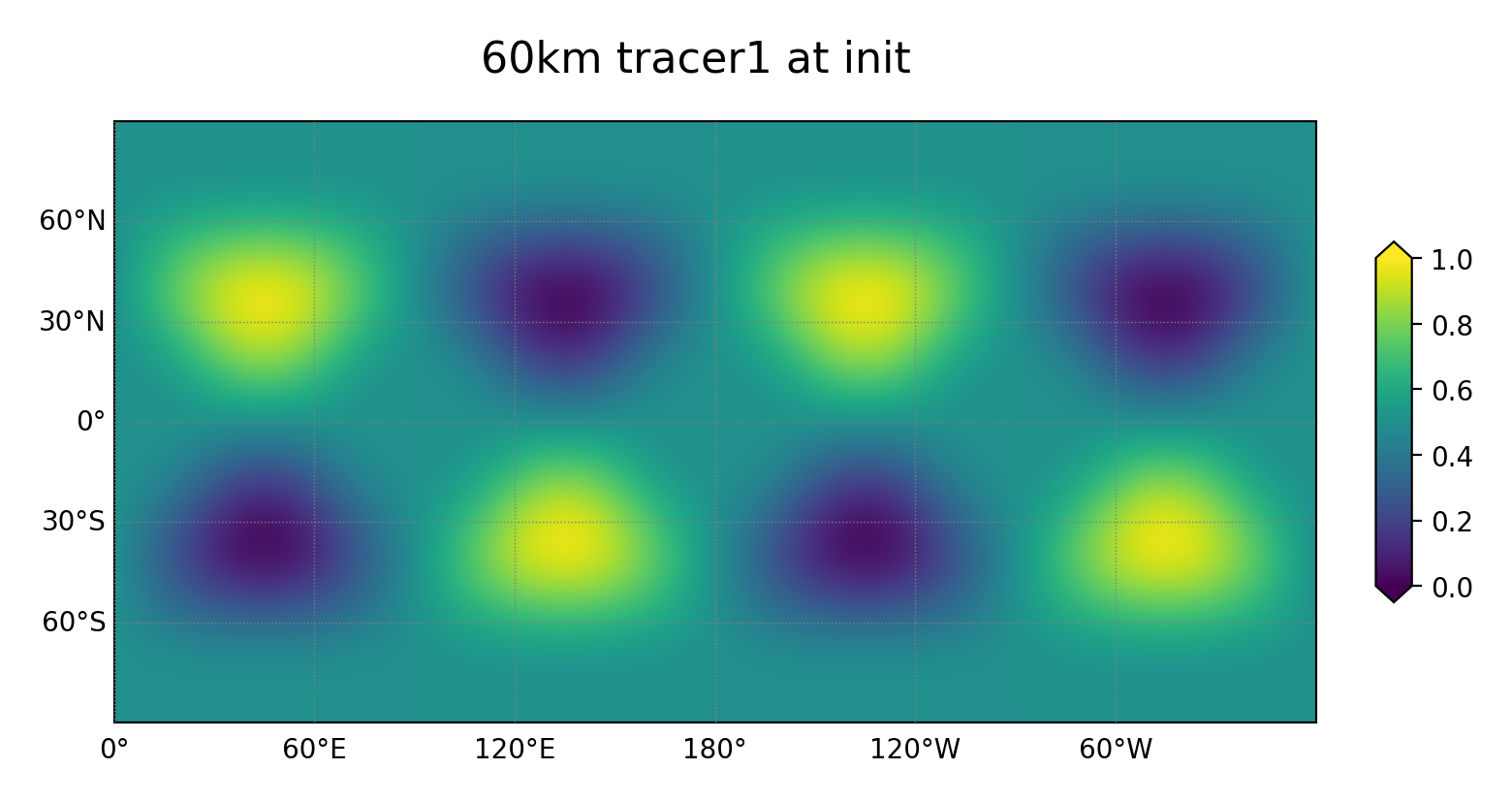
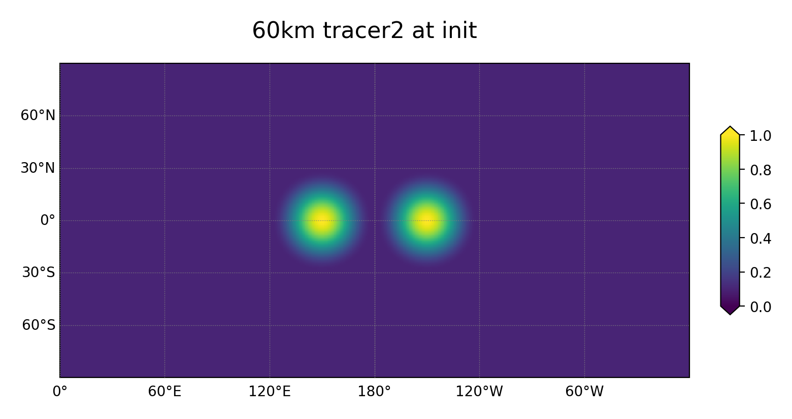
initial conditions

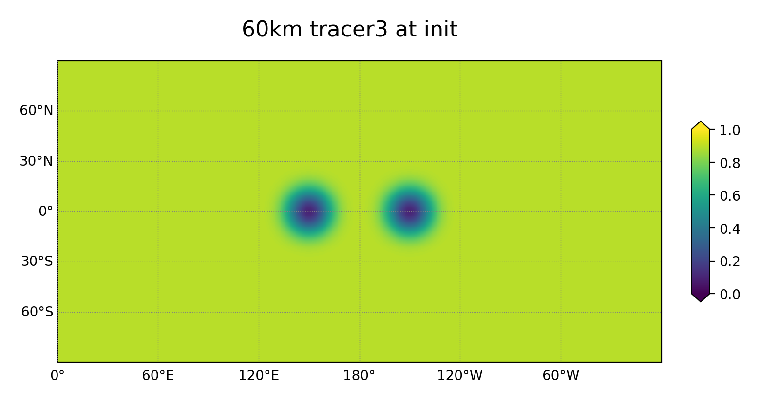
The initial condition is characterized by three separate tracer distributions stored in three debugTracers:

tracer1: A c-infinity function used for convergence analysis
tracer2: A pair of c-2 cosine bells
tracer3: A second pair of cosine bells that are nonlinearly correlated with tracer2.

../../../_images/correlated_tracers_2d_init_tracer1.png

../../../_images/correlated_tracers_2d_init_tracer2.png

../../../_images/correlated_tracers_2d_init_tracer3.png

The velocity is

\[ u(t) = \frac{10 R}{\tau} \sin^2(\lambda - \frac{2 \pi t}{\tau}) \sin(2\theta) \cos(\frac{\pi t}{\tau}) + \frac{2 \pi R}{\tau}\cos(\theta) \]

\[ v(t) = \frac{10 R}{\tau} \sin(2\lambda - \frac{4 \pi t}{\tau}) \cos(\theta) \cos(\frac{\pi t}{\tau}) \]

Where $\lambda$ is longitude, $\theta$ is latitude and $R$ is the radius of the sphere. $\tau$ is the time it takes to transit the equator. The default is 12 days and is given by the cfg option vel_pd.

Temperature and salinity are not evolved in this task and are given constant values determined by config options temperature and salinity.

The Coriolis parameters fCell, fEdge, and fVertex do not need to be specified for a global mesh and are initialized as zeros.

forcing

This case is forced to follow $u(t)$ and $v(t)$ given above.

time step and run duration

This task uses the Runge-Kutta 4th-order (RK4) time integrator. The time step for forward integration is determined by multiplying the resolution by a config option, rk4_dt_per_km, so that coarser meshes have longer time steps. You can alter this before setup (in a user config file) or before running the task (in the config file in the work directory).

# config options for spherical convergence tests
[spherical_convergence_forward]

# time integrator: {'split_explicit', 'RK4'}
time_integrator = RK4

# RK4 time step per resolution (s/km), since dt is proportional to resolution
rk4_dt_per_km = 3.0

The convergence_eval_time, run_duration and output_interval are the period for advection to make a full rotation around the globe, 12 days:

# config options for spherical convergence tests
[spherical_convergence_forward]

# Run duration in days
run_duration = ${sphere_transport:vel_pd}

# Output interval in days
output_interval = ${sphere_transport:vel_pd}

Here, ${sphere_transport:vel_pd} means that the same value is used as in the option vel_pd in section [sphere_transport], see below.

config options

The correlated_tracer_2d config options include:

# options for all sphere transport test cases
[sphere_transport]

# temperature
temperature = 15.

# salinity
salinity = 35.

# time (hours) for bell to transit equator once
vel_pd = 288.0

# radius of cosine bells tracer distributions
cosine_bells_radius = 0.5

# background value of cosine bells tracer distribution
cosine_bells_background = 0.1

# amplitude of cosine bells tracer distribution
cosine_bells_amplitude = 0.9

# radius of slotted cylinders tracer distributions
slotted_cylinders_radius = 0.5

# background value of slotted cylinders tracer distribution
slotted_cylinders_background = 0.1

# amplitude of slotted cylinders tracer distribution
slotted_cylinders_amplitude = 1.0


# options for tracer visualization for the sphere transport test case
[sphere_transport_viz_tracer]

# colormap options
# colormap
colormap_name = viridis

# the type of norm used in the colormap
norm_type = linear

# colorbar limits
colorbar_limits = 0., 1.


# options for plotting tracer differences from sphere transport tests
[sphere_transport_viz_tracer_diff]

# colormap options
# colormap
colormap_name = cmo.balance

# the type of norm used in the colormap
norm_type = linear

# colorbar limits
colorbar_limits = -0.25, 0.25


# options for thickness visualization for the sphere transport test case
[sphere_transport_viz_h]

# colormap options
# colormap
colormap_name = viridis

# the type of norm used in the colormap
norm_type = linear

# colorbar limits
colorbar_limits = 99., 101.


# options for plotting tracer differences from sphere transport tests
[sphere_transport_viz_h_diff]

# colormap options
# colormap
colormap_name = cmo.balance

# the type of norm used in the colormap
norm_type = linear

# colorbar limits
colorbar_limits = -0.25, 0.25


# options for correlated tracers 2-d test case
[correlated_tracers_2d]

# velocity amplitude in meters per second
vel_amp = 10.

# convergence threshold below which the test fails
convergence_thresh_tracer1 = 1.7
convergence_thresh_tracer2 = 1.66
convergence_thresh_tracer3 = 1.28

# time in days at which to evaluate mixing
mixing_evaluation_time = 6.0

The options in section sphere_transport are used by all 4 test cases based on Lauritzen et al. (2012) and control the initial condition. The options in section correlated_tracers_2d control the initial condition of that case only, the convergence rate threshold, and the time at which to evaluate mixing diagnostics.

The options in sections sphere_transport_viz* control properties of the viz step of the test case.

The default options for the convergence analysis step can be changed here:

# config options for spherical convergence tests
[spherical_convergence]

# Evaluation time for convergence analysis (in days)
convergence_eval_time = ${sphere_transport:vel_pd}

# Type of error to compute
error_type = l2

cores

The target and minimum number of cores are determined by goal_cells_per_core and max_cells_per_core from the ocean section of the config file, respectively. This ensures that the number of cells per core is roughly constant across the different resolutions in the convergence study.