geostrophic

description

The geostrophic tasks implement the “Global Steady State Nonlinear Zonal Geostrophic Flow” test case described in Williamson et al. 1992

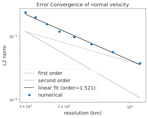
The task geostrophic/convergence_both is a space-and-time convergence test with time step varying proportionately to grid size. Convergence tests in either space or time are also available as convergence_space or convergence_time. The result of the analysis step of the task are plots like the following showing convergence of water-column thickness and normal velocity as functions of the mesh resolution:

Visualizations of the fields themselves can be added in viz steps by appending with_viz to the task name at setup.

suppported models

These tasks support only MPAS-Ocean.

mesh

The mesh is global and can be constructed either as quasi-uniform or icosahedral. At least three resolutions must be chosen for the mesh convergence study. The base meshes are the same as used in cosine bell. See cosine bell’s mesh section for more details.

vertical grid

This test case only exercises the shallow water dynamics. As such, the minimum number of vertical levels may be used. The bottom depth is constant and the results should be insensitive to the choice of bottom_depth. See cosine bell’s vertical grid section for the config options.

initial conditions

The steady-state fields are given by the following equations:

\[\begin{split} u & = u_0 (\cos\theta \cos\alpha + \cos\lambda \sin\theta \sin\alpha)\\ v & = -u_0 \sin\lambda \sin\alpha\\ h & = h_0 - 1/g (a \Omega u_0 + u_0^2/2)(-\cos\lambda \cos\theta \sin\alpha + \sin\theta \cos\alpha)^2 \end{split}\]

where

\[\begin{split} u_0 & = 2 \pi a/(12 \textrm{ days})\\ h_0 & = (1/g) \, 2.94 \times 10^{4} \textrm{m}^2/\textrm{s}^2 \\ \alpha & = 0 \end{split}\]

In this test case, the initial fields are given their steady-state values and the simulation should not diverge significantly from those values.

In this test case, the bottom topography is flat so initial conditions are given for bottomDepth and ssh such that h = bottomDepth + ssh.

The initial conditions also includes the coriolis parameter, given as:

\[ f = 2 \Omega (-\cos\lambda \cos\theta \sin\alpha + \sin\theta \cos\alpha) \]

In future work, alpha may be varied to test the sensitivity to orientation:

\[ \alpha = [0, 0.05, \pi/2 - 0.05, \pi/2] \]

forcing

Probably N/A but see Williamson’s text about the possibility of prescribing a wind field.

time step and run duration

This task uses the Runge-Kutta 4th-order (RK4) time integrator. The time step for forward integration is determined by multiplying the resolution by a config option, rk4_dt_per_km, so that coarser meshes have longer time steps. You can alter this before setup (in a user config file) or before running the task (in the config file in the work directory).

# config options for convergence tests
[convergence_forward]

# time integrator: {'split_explicit', 'RK4'}
time_integrator = RK4

# RK4 time step per resolution (s/km), since dt is proportional to resolution
rk4_dt_per_km = 2.0

The convergence_eval_time, run_duration and output_interval are all 5 days (120 hours):

# config options for convergence tests
[convergence]

# Evaluation time for convergence analysis (in hours)
convergence_eval_time = 120.0

# config options for convergence forward steps
[convergence_forward]

# Run duration in hours
run_duration = ${convergence:convergence_eval_time}

# Output interval in hours
output_interval = ${run_duration}

Here, ${convergence:convergence_eval_time} means that the same value is used as in the option convergence_eval_time in section [convergence].

analysis

For analysis we compute the \(l_1\), \(l_2\) and \(l_{\inf}\) error norms of h and velocity relative to the steady-state solutions given above.

First, each of these errors norms are plotted vs time for a given resolution.

Then, mesh convergence is examined by plotting the \(l_2\) and \(l_{\inf}\) norms at day 5 vs resolution.

config options

The geostrophic config options include:

# options for geostrophic convergence test case
[geostrophic]

# period of the velocity in days
vel_period = 12.0

# reference water column thickness (m^2/s^2)
gh_0 = 2.94e4

# angle of velocity field variation
alpha = 0.0

# the constant temperature of the domain
temperature = 15.0

# the constant salinity of the domain
salinity = 35.0

These are the basic constants used to initialize the test case according to the Williams et al. (1992) paper. The temperature and salinity are arbitrary, since they do not vary in space and should not affect the evolution.

Three additional config options relate to detecting when the convergence rate for the water-column thickness (h) and normal velocity (using the L2 norm to compute the error). If either convergence rate is unexpectedly low an error is raised:

# config options for convergence tests
[convergence]

# Type of error to compute
error_type = l2

# options for geostrophic convergence test case
[geostrophic]

# convergence threshold below which the test fails
convergence_thresh_h = 0.4
convergence_thresh_normalVelocity = 1.3

The convergence rate of the water-column thickness for this test case is very low for the QU meshes in MPAS-Ocean, about 0.5, which necessitates the very generous convergence threshold used here.

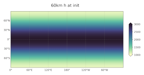
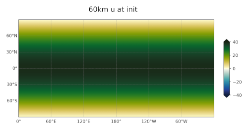
Config options related to visualization are as follows. The options in geostropnic_viz are related to remapping to a regular latitude-longitude grid. The remaining options are related to plotting water-column thickness (h) and velocities (u and v) and the difference between these fields at initialization and after the 5-day run.

# options for plotting water-column thickness from the geostrophic test
[geostrophic_viz_h]

# colormap options
# colormap
colormap_name = cmo.deep

# the type of norm used in the colormap
norm_type = linear

# colorbar limits
colorbar_limits = 1000.0, 3000.0

# colorbar label
label = water-column thickness (m)

# options for plotting velocity from the geostrophic test
[geostrophic_viz_vel]

# colormap options
# colormap
colormap_name = cmo.delta

# the type of norm used in the colormap
norm_type = linear

# colorbar limits
colorbar_limits = -40.0, 40.0

# colorbar label
label = velocity (m/s)

# options for plotting water-column thickness from the geostrophic test
[geostrophic_viz_diff_h]

# colormap options
# colormap
colormap_name = cmo.balance

# the type of norm used in the colormap
norm_type = linear

# colorbar limits
colorbar_limits = -10.0, 10.0

# colorbar label
label = water-column thickness (m)

# options for plotting velocity from the geostrophic test
[geostrophic_viz_diff_vel]

# colormap options
# colormap
colormap_name = cmo.balance

# the type of norm used in the colormap
norm_type = linear

# colorbar limits
colorbar_limits = -0.3, 0.3

# colorbar label
label = velocity (m/s)

cores

The number of cores for each step is handled in the same way as the cosine bell test. See that test’s cores section for details.