horizontal pressure gradient

description

The horiz_press_grad tasks in polaris.tasks.ocean.horiz_press_grad exercise Omega’s hydrostatic pressure-gradient acceleration (HPGA) for a two-column configuration with prescribed horizontal gradients.

The analysis uses two different baselines, each with a different purpose:

• an analytic reference solution evaluated inside the analysis step that is used as the main accuracy target, and

• a Python-computed two-column HPGA diagnostic from the init step that is used as a consistency check against Omega.

Each task includes:

• an init step at each horizontal/vertical resolution pair,

• a single-time-step forward run at each horizontal resolution, and

• an analysis step that evaluates the analytic reference and compares Omega output with both the reference and the Python-initialized HPGA.

The tasks currently provided are:

ocean/column/horiz_press_grad/salinity_gradient
ocean/column/horiz_press_grad/temperature_gradient
ocean/column/horiz_press_grad/ztilde_gradient

The point of these tasks is not only to verify that Omega can reproduce the same discrete answer as the Python initialization, but also to measure how the two-column discretization converges toward a more accurate non-local approximation of the continuous hydrostatic pressure-gradient force.

supported models

These tasks currently support Omega only.

mesh

The mesh is planar with two adjacent ocean cells. For each resolution in horiz_resolutions, the spacing between the two columns is set by that value (in km).

The HPGA diagnostic is evaluated on the single internal horizontal edge that connects the two columns, at each layer midpoint. In this page, x denotes the along-layer horizontal direction used by Omega’s horizontal gradient operator. In the idealized two-column planar geometry, this direction follows the line joining the two cell centers. It is therefore related to the shared edge normal, but it is not intended to define a separate exact geometric edge-normal coordinate.

vertical grid

The vertical coordinate is p-star (see p-star), Omega’s ALE pseudo-compressible variant of the z-tilde coordinate, with a uniform pseudo-height spacing for each test in vert_resolutions.

The meaning of the along-layer x direction depends on the task variant. In the salinity_gradient and temperature_gradient tests, the z-tilde interfaces are level, so pressure surfaces are also horizontally level except where they intersect the bathymetry. In the ztilde_gradient test, the prescribed z-tilde gradient tilts the layers, so the pressure surfaces are sloped and the along-layer direction follows those sloping layers.

reference solution

The reference HPGA is evaluated analytically at the edge (\(x = 0\)) using the chain-rule / Leibniz expansion of the horizontal pressure-gradient force in pseudo-height coordinates. Because the continuous pressure-gradient force is coordinate-invariant, the along-pseudo-height formula equals \(-g\,\partial z / \partial x\big|_{\tilde z}\) exactly, including near the seafloor.

The reference is anchored at the surface rather than the seafloor, because the surface is the boundary the model honours: Init/Omega build the p-star column from the prescribed sea-surface height and surface pressure, so the HPGA vanishes at the surface (for zero surface slope) and grows downward.

The reference acceleration at pseudo-height \(\tilde z\) is

\[ a(\tilde z) = -g\left[\eta' - \rho_0\,\alpha(\tilde z_s)\,\tilde z_s' + \rho_0 \int_{\tilde z_s}^{\tilde z} \bigl(\alpha_{S_A}\,\partial_x S_A + \alpha_{\Theta}\,\partial_x \Theta\bigr)\, d\tilde z'\right], \]

where:

• \(\eta' = \partial_x \eta\) is the sea-surface-height gradient,

• \(\tilde z_s\) is the surface pseudo-height (\(\tilde z_s = -p_s / (\rho_0 g)\), zero only when the surface pressure is zero) and \(\tilde z_s' = \partial_x \tilde z_s\) is its gradient,

• \(\alpha\) is specific volume from the TEOS-10 equation of state,

• \(\alpha_{S_A} = \partial \alpha / \partial S_A\) and \(\alpha_{\Theta} = \partial \alpha / \partial \Theta\) are TEOS-10 first derivatives of specific volume.

The surface boundary term is kept fully general, so a nonzero sea-surface height or surface pressure (nonzero geom_ssh_grad and/or surface z_tilde_grad node) is supported without further changes. The three task variants currently provided all use zero surface slope.

The gradients \(\partial_x S_A\) and \(\partial_x \Theta\) at fixed \(\tilde z\) are obtained by centred finite-differencing PCHIP interpolants evaluated at \(x = \pm\varepsilon\), where \(\varepsilon =\) reference_horiz_eps_km (1 m by default). This handles moving-node inputs correctly, so it is valid for the ztilde_gradient task as well as the level-layer tasks.

The integral in the formula is evaluated by composite quadrature. The number of sub-panels per interval is set by reference_quadrature_subdivisions (4 by default).

For comparison with a layer-averaged Omega tendency, the analysis step averages \(a(\tilde z)\) over the model’s actual pseudo-height layer bounds using 4-point Gauss–Legendre quadrature with reference_quadrature_subdivisions sub-panels per layer. The deepest valid layer (which abuts the bathymetry) is excluded from the RMS error calculation, because partial bottom cells make that layer’s geometric extent differ from the smooth reference geometry.

python HPGA in the init step

The init step computes a second HPGA estimate directly from the initialized two-column state. This calculation is intentionally much closer to the discrete Omega formulation than the high-fidelity reference is.

First, the step constructs the two-cell mesh and the test vertical grid for the requested (horiz_res, vert_res) pair. Because the geometric water-column thickness depends on the equation of state through the mapping from z-tilde to geometric height, the step iteratively rescales the pseudo-bottom depth so that the resulting geometric water-column thickness matches the prescribed sea-surface and bottom geometry. This fixed-point iteration is provided by polaris.ocean.vertical.pstar_init.PStarInitStep (see Vertical coordinate), from which Init inherits.

Once the initialized state is available, the Python diagnostic computes the same thermodynamic quantities used by Omega: pressure, specific volume, geometric height, and Montgomery potential. It then forms a two-column finite difference,

\[ \frac{\partial M}{\partial x} \approx \frac{M_R - M_L}{\Delta x}, \qquad \frac{\partial \alpha}{\partial x} \approx \frac{\alpha_R - \alpha_L}{\Delta x}, \]

with edge pressure

\[ p_{\mathrm{edge}} = \frac{p_L + p_R}{2}, \]

and writes the corresponding diagnostic

\[ \mathrm{HPGA}_{\mathrm{python}} = -\frac{\partial M}{\partial x} + p_{\mathrm{edge}}\frac{\partial \alpha}{\partial x} \]

to init.nc.

This Python HPGA is not the main reference solution. Instead, it checks whether Omega’s one-step tendency matches the expected two-column discrete calculation from the initialized state.

config options

Shared options are in section [horiz_press_grad]:

# resolutions in km (distance between the two columns)
horiz_resolutions = [4.0, 3.0, 2.0, 1.5, 1.0, 0.75, 0.5]

# vertical resolution in m for each two-column setup
vert_resolutions = [4.0, 3.0, 2.0, 1.5, 1.0, 0.75, 0.5]

# geometric sea-surface and sea-floor midpoint values and x-gradients
geom_ssh_mid = 0.0
geom_ssh_grad = 0.0
geom_z_bot_mid = -500.0
geom_z_bot_grad = 0.0

# pseudo-height bottom midpoint and x-gradient
z_tilde_bot_mid = -576.0
z_tilde_bot_grad = 0.0

# midpoint and gradient node values for piecewise profiles
z_tilde_mid = [0.0, -48.0, -144.0, -288.0, -576.0]
z_tilde_grad = [0.0, 0.0, 0.0, 0.0, 0.0]

temperature_mid = [22.0, 20.0, 14.0, 8.0, 5.0]
temperature_grad = [0.0, 0.0, 0.0, 0.0, 0.0]

salinity_mid = [35.6, 35.4, 35.0, 34.8, 34.75]
salinity_grad = [0.0, 0.0, 0.0, 0.0, 0.0]

# reference settings
reference_quadrature_method = gauss4
reference_quadrature_subdivisions = 4
reference_horiz_eps_km = 1.0e-3

# regression thresholds and convergence checks
omega_vs_polaris_rms_threshold = 1.0e-10
omega_vs_reference_high_res_rms_threshold = 1.0e-6
omega_vs_reference_convergence_rate_min = 1.5
omega_vs_reference_convergence_rate_max = 2.1
omega_vs_reference_convergence_fit_max_resolution = 4.0

The omega_vs_polaris_rms_threshold bounds the RMS difference between the Omega forward HPGA and the Python-initialized HPGA (the consistency check). The omega_vs_reference_* options bound the Omega-vs-reference accuracy: the RMS error at the highest resolution, the allowed power-law convergence slope, and the finest horizontal resolution included in the convergence fit (all resolutions are still shown in the plots).

The three task variants specialize one horizontal gradient field:

• salinity_gradient: nonzero salinity_grad

• temperature_gradient: nonzero temperature_grad

• ztilde_gradient: nonzero z_tilde_bot_grad

time step and run duration

The forward step performs one model time step and outputs pressure-gradient diagnostics used in the analysis.

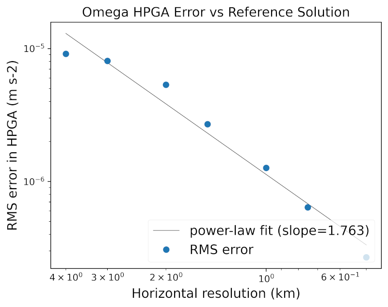
analysis

The analysis step computes and plots:

• Omega RMS error versus reference (omega_vs_reference.png), including a power-law fit and convergence slope, and

• Omega RMS difference versus Python initialization (omega_vs_python.png).

The corresponding tabulated data are written to omega_vs_reference.nc and omega_vs_python.nc.

For the Omega-versus-reference comparison, the analytic reference \(a(\tilde z)\) is layer-averaged over the model’s actual pseudo-height layer bounds (from init.nc) using 4-point Gauss–Legendre quadrature. The deepest valid layer is excluded from the RMS error calculation because that layer abuts the bathymetry, where partial bottom cells make the model layer’s geometric extent differ from the smooth reference geometry.

For the Omega-versus-Python comparison, the analysis uses the HPGA written by the init step in init.nc, so this second metric should be read as an implementation-consistency check rather than as an accuracy measure against the high-fidelity reference.

Implementation details for the ReferenceColumn evaluator and the init and analysis steps are described in horiz_press_grad.