Quick guide for LLNL AIMS4 or ACME1 (v1)
If you’re pressed for time, just follow this quick guide to
run e3sm_diags on aims4 or acme1.
Log on to
aims4:
ssh -Y aims4.llnl.gov
or acme1:
ssh -Y acme1.llnl.gov
2. If you don’t have Anaconda installed, follow this guide.
Make sure you are using
bash
bash
Installing and creating an environment
The steps below detail how to create your own environment with e3sm_diags.
However, it is possible to use the E3SM Unified Environment instead.
If you decide to use the unified environment, please do so and skip to step 5.
Allow Anaconda to download packages, even with a firewall.
conda config --set ssl_verify false
binstar config --set verify_ssl False
Update Anaconda.
conda update conda
Get the yml file to create an environment.
wget https://raw.githubusercontent.com/E3SM-Project/e3sm_diags/master/conda/e3sm_diags_env.yml
Remove any cached Anaconda packages. This will ensure that you always get the latest packages.
conda clean --all
8. Use Anaconda to create a new environment with e3sm_diags installed.
Tip: You can change the name of the environment by adding -n new_env_name to the end of conda env create ....
conda env create -f e3sm_diags_env.yml
source activate e3sm_diags_env
Running the entire Latitude-longitude contour set
9. Copy and paste the below code into myparams.py using your
favorite text editor. Adjust any options as you like.
reference_data_path = '/p/cscratch/acme/data/obs_for_e3sm_diags/climatology/'
test_data_path = '/p/cscratch/acme/data/test_model_data_for_acme_diags/climatology/'

test_name = '20161118.beta0.FC5COSP.ne30_ne30.edison'

sets = ["lat_lon"]

backend = 'mpl'  # 'mpl' is for the matplotlib plots.

results_dir = 'lat_lon_demo'  # name of folder where all results will be stored

multiprocessing = True
num_workers = 16  # Number of processes to use
Run the diags.
e3sm_diags -p myparams.py
Open the following webpage to view the results.
firefox --no-remote lat_lon_demo/viewer/index.html &
The
--no-remoteoption uses the Firefox installed on this machine, and not the one on your machine.
Tip: Once you’re on the webpage for a specific plot, click on the ‘Output Metadata’ drop down menu to view the metadata for the displayed plot.
Running that command allows the displayed plot to be recreated. Changing any of the options will modify the resulting figure.
Running all of the diagnostics sets
12. To run all of the diagnostic sets that this software supports, open myparams.py
and remove the sets parameter. If should look like this:
reference_data_path = '/p/cscratch/acme/data/obs_for_e3sm_diags/climatology/'
test_data_path = '/p/cscratch/acme/data/test_model_data_for_acme_diags/climatology/'

test_name = '20161118.beta0.FC5COSP.ne30_ne30.edison'

# When commented out, this is ignored.
# We can also just delete this line.
# sets = ["lat_lon"]

backend = 'vcs'  # 'mpl' is for the matplotlib plots.

results_dir = 'lat_lon_demo'  # name of folder where all results will be stored

multiprocessing = True
num_workers = 16  # Number of processes to use
13. Now run and view the results. This will take some more time, so if you can,
change the num_workers parameter to use more processors so it can be faster!
e3sm_diags -p myparams.py
firefox --no-remote lat_lon_demo/viewer/index.html &
Advanced: Running custom diagnostics
The following steps are for ‘advanced’ users, who want to run custom diagnostics. So most users will not run the software like this.
14. By default, all of the E3SM diagnostics are ran for the sets that
we defined above. This takes some time, so we’ll create our own
diagnostics to be ran. Run the command
touch mydiags.cfg
and paste the code below in mydiags.cfg. Check defining parameters
for all available parameters.
[#]
case_id = "GPCP_v2.2"
variables = ["PRECT"]
ref_name = "GPCP_v2.2"
reference_name = "GPCP (yrs1979-2014)"
seasons = ["ANN", "DJF"]
regions = ["global"]
test_colormap = "WhiteBlueGreenYellowRed.rgb"
reference_colormap = "WhiteBlueGreenYellowRed.rgb"
diff_colormap = "BrBG"
contour_levels = [0.5, 1, 2, 3, 4, 5, 6, 7, 8, 9, 10, 12, 13, 14, 15, 16]
diff_levels = [-5, -4, -3, -2, -1, -0.5, 0.5, 1, 2, 3, 4, 5]

[#]
case_id = "SST_CL_HadISST"
variables = ["SST"]
ref_name = "HadISST_CL"
reference_name = "HadISST/OI.v2 (Climatology) 1982-2001"
seasons = ["ANN", "MAM"]
contour_levels = [-1, 0, 1, 3, 6, 9, 12, 15, 18, 20, 22, 24, 26, 28, 29]
diff_levels = [-5, -4, -3, -2, -1, -0.5, -0.2, 0.2, 0.5, 1, 2, 3, 4, 5]
Run the custom diagnostics.
e3sm_diags -p myparams.py -d mydiags.cfg
Open the following webpage to view the results.
firefox --no-remote lat_lon_demo/viewer/index.html &
More Options
You can modify the
setsparameters inmyparams.pyto run multiple sets. Possible options are:'zonal_mean_xy', 'zonal_mean_2d', 'lat_lon, 'polar', 'cosp_histogram'. If thesetsparameter is not defined, all of the aforementioned sets are ran. Ex:sets = ['zonal_mean_xy', 'zonal_mean_2d', 'lat_lon', 'polar', 'cosp_histogram']
Diagnostics can be ran in parallel with multi-processing. In
myparams.py, addmultiprocessing = Trueand setnum_workersto the number of workers you want to use. Ifnum_workersis not defined, it will automatically use 4 processors processes by default on a machine. Ex:# myparams.py # In addition to your other parameters, include: multiprocessing = True num_workers = 4
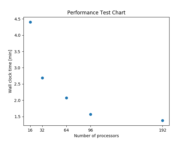
Below figure shows a scalability test running the package for all lat_lon diagnostics on ACME1. Courtesy of Sterling Baldwin.

Performance test running the package with full set: “lat_lon” diagnostics on ACME1